This blog post describes the experiences of using the freely available Python- and web-clients to the VirES for Swarm (more information here (opens new window)) interface that provides highly interactive data manipulation and retrieval interface for ESA’s Swarm constellation mission science products (more information here (opens new window)). The idea was to test the new service (for more details read a blog post by Ashley Smith) provided by EOX that allows user very simple and flexible access to data, e.g., Swarm mission data, and perform fast visualisation of the different scientific products.

ESA’s Swarm Constellation Mission Data Access

All the three Swarm satellite are equipped with a set of identical instruments: absolute scalar and vector field magnetometers; star tracker; electric field instrument; GPS receiver; laser retro-reflector and accelerometer (more information here (opens new window)). This instrumentation allows achieving the main science objectives of the mission: studies of core dynamics, geodynamo processes and core-mantle interaction; mapping of the lithospheric magnetisation and its geological interpretation; determination of the 3D electrical conductivity of the mantle; investigation of electric currents flowing in the magnetosphere and ionosphere. The amount of scientific products is increasing from year to year and covers quite a wide range of measurements and models (more information here (opens new window)). All these products/data are freely accessible to all users via anonymous access in accordance with ESA Earth Observation Data Policy via any HTTP browser (http://swarm-diss.eo.esa.int (opens new window)) and an ftp client (ftp://swarm-diss.eo.esa.int).

VirES Web-Client Visualisation tools for Swarm Products

The VirES web-client provides an excellent opportunity of Swarm data visualization in a fast and effective way and produces the publication-ready graphics and charts through an intuitive, powerful and customizable interface that immediately take effect on the display. The plot below is an example of such time-efficient plot production of Swarm orbits for one given day over the globe to illustrate the spatial coverage of all three satellites.

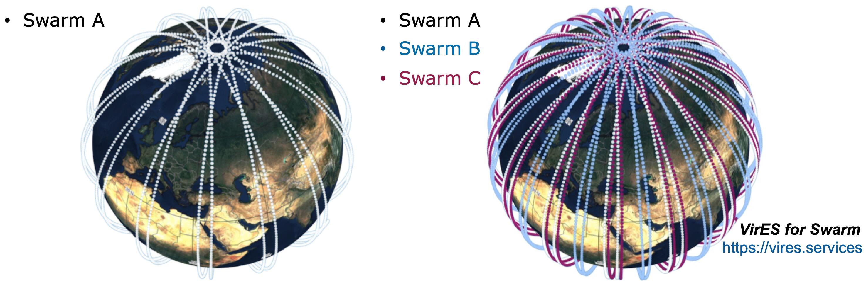
Screenshot from the talk given to the broad audience

The “normal” way to produce this or other plots would be, first to access and download Swarm data (ftp or http); second to read, e.g., the CDF file information or data handbook (available here (opens new window)) for the given product; third to write script or code to read and process the date and than as a last step visualize it (also very time consuming). And this was an “easy” example where no model calculations were involved that would make this process even longer. The VirES web-client, however, provides a tool for an efficient way for visualisation that does not request user knowledge on additional data included in the file to be visualised or how to combine different data files to get a final plot for publication or presentation purposes. Additionally, VirES allows data download that can be combined to fit various use cases. All this is achieved in a user-friendly environment with powerful and intuitive built-in visualisation tools.

VirES Python-Client programmatic package for Swarm Products

The VirES Python-client-module provides a good possibility of programmatic access to the VirES-server. Namely, this module serves as the application programming interface (API) and allows users to access VirES database of Swarm data products and offers opportunities for various model calculations. For this activity, I have used a Jupiter notebook environment, and tested the advantage to allow users to work in parallel and share codes and data.

VirES offers several build in models, e.g., MCO_SHA_2C (use example here (opens new window)), but for this case, it was important to import my user-defined models of the Earth’s magnetic field, e.g., core field and lithospheric field. In the VirES client, it is possible to import users’ own models. Therefore, the first step was to upload the spherical harmonic coefficients from external files. For this purpose, the models AUX_CORE and AUX_LIT (not available publicly, but accessible for DISC members) have been used. These models are also applied for calculating the Swarm Level 2 Ionospheric Radial Current (IRC) and Ionospheric Bubble Index (IBI) products (more information here (opens new window)). I have used the following Python script to upload these models:

from viresclient import SwarmRequest
from pylab import *
import datetime as dt
from eoxmagmod import load_model_shc

corePath = '../share/jan.rauberg/SW_OPER_AUX_COR_2__20131126T000000_20190101T000000_0001.DBL'
litPath = '../share/jan.rauberg/SW_OPER_AUX_LIT_2__00000000T000000_99999999T999999_0003.DBL'
core_model = load_model_shc(corePath)
lit_model  = load_model_shc(litPath)

Next, I requested the magnetic field data for the given Swarm satellite (e.g., Swarm A on 5 July, 2017) from VirES server:

request = SwarmRequest(url="https://staging.viresdisc.vires.services/openows")
request.set_collection("SW_OPER_MAGA_LR_1B")
request.set_products(measurements=["B_NEC", "F"], sampling_step="PT1S")
tss = dt.datetime(2017,7,5)
tse = dt.datetime(2017,7,6)
ds = request.get_between(start_time=tss, end_time=tse).as_xarray()

The following lines of code show an example how to evaluate the uploaded models, in this case AUX_CORE and AUX_LIT:

core = core_model.eval(mjd2k, pos, scale=[1, 1, -1])
#note the reversed radial component
lit  = lit_model.eval(mjd2k, pos, scale=[1, 1, -1])

Note that these are only parts of the Python script, which uses designated VirES services. The following plot show the magnetic field residuals calculate as:

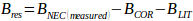
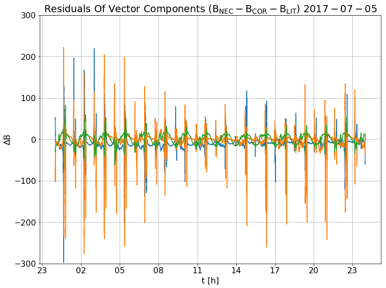
Screenshot of residual magnetic field calculated with VirES client

Based on these results, it was rather straightforward to extend the Python script for Ionospheric Radial Current (IRC) calculations for the single satellite case. However, these calculated IRCs are a reduced version of the official Swarm L2 IRC product since the model for the magnetospheric field is not considered. The comparison plot between the reduced model family to calculate IRC, one using the VirES client and other from original code (also without magnetospheric part), is shown below.

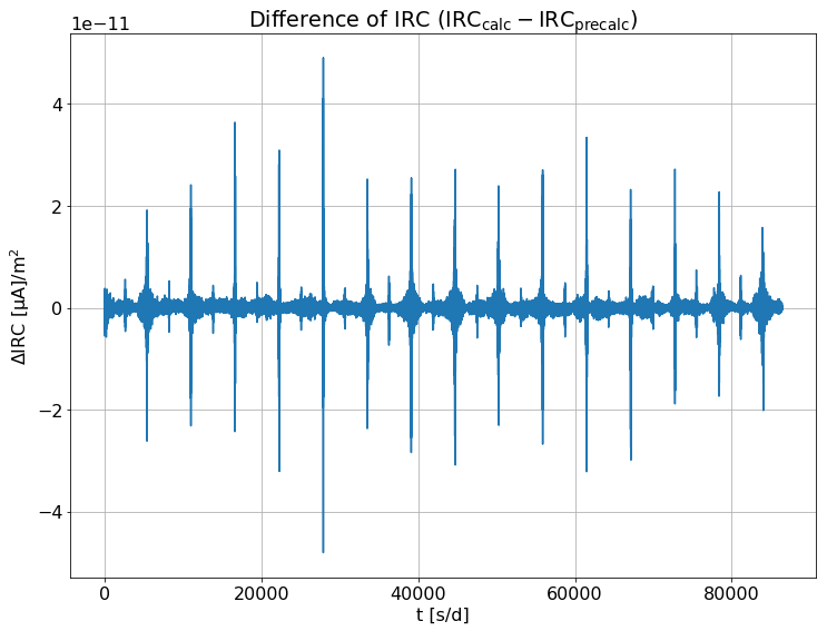
Screenshot of the difference between the two codes used to calculate IRC

The original amplitudes of the IRCs are about 0.01-10 mA/m^2. Hence, the differences between the two methods are very close to the noise level. This concludes that the implemented VirES tool provide reasonable and good results and can be offered for public use.